One hugely important area in which my knowledge is close to zero is machine learning and artificial intelligence. It’s not only a terrible but also pitiful idea to finish a graduate degree in computer science without knowing at least somewhat how this stuff works, so I decided to follow the openly available Stanford CS229 machine learning course and provide a summary for each chapter here since exercise material and lecture notes appear to have been taken down. I try to apply as much as possible and follow along using Rust. The code can be found under Baseng0815/ml-implementations.
Linear regression allows us to make predictions by training a model on a given set of training data and then applying this model to new values. More formally, given training data in the form of \(m\) pairs \((x^{(i)},y^{(i)})\) of feature vectors \(x^{(i)}\in\mathbb{R}^d\) and values \(y^{(i)}\in\mathbb{R}\), we try to find parameters \(\theta\) so that the prediction function \(h_\theta:\mathbb{R}^d\rightarrow\mathbb{R}\) is as accurate as possible w.r.t. some loss metric \(\mathcal{J}:\theta\rightarrow\mathbb{R}\):
\[\begin{gather} arg\min_\theta\mathcal{J(\theta)} \end{gather}\]
Now the question of how to choose \(h_\theta\) and \(\mathcal{J}\) naturally arises. Since we are doing linear regression, we will choose a linear model which will make a prediction by linear combination of features using weights \(\theta_i\). To account for bias, we will also add a dummy feature \(x_0=1\) so that \(\theta_0 x_0=\theta_0\). Conveniently, this allows us to rewrite predictions as matrix-vector multiplication and opens the door to all the neat linear algebra tools:
\[\begin{gather} h_\theta(x)=\sum_{j=0}^d \theta^{(i)}x^{(i)}=\theta^Tx^{(i)} \end{gather}\]
The loss metric usually employed is mean-squared error (MSE) which is defined as follows:
\[\begin{gather} \mathcal{J}(\theta)=\frac{1}{m}\sum_{i=1}^d\mathcal{J}_{x^{(i)}}(\theta)=\frac{1}{m}\sum_{i=1}^d (h_\theta(x^{(i)})-y^{(i)})^2 \end{gather}\]
Why did we define the loss metric this way? The simple answer you might have already come across is that we want to avoid negative loss values and taking the absolute value is bad since it leaves \(\mathcal{J}\) non-continuous and thus non-differentiable. This explanation alone (at least for me) was unsatisfactory since we could have also chosen \(\mathcal{J}_{x^{(i)}}(\theta)=(h_\theta(x^{(i)})-y^{(i)})^4\) or basically any other positive, differentiable function. A more technical explanation can be found in the assumption of the distribution of noise in the data. Since almost all real-life data exhibits some form of measuring error and other unmodeled randomness, our prediction can never be fully accurate. Let \(\Sigma^{(i)}\) denote the error terms; the true situation then looks like this:
\[\begin{gather} y^{(i)}=\theta^{(i)}x^{(i)}+\Sigma^{(i)} \end{gather}\]
We now assume \(\Sigma^{(i)}\) to be iid (independently and identically distributed) following a Gaussian distribution with mean \(\mu=0\) and some unknown standard deviation \(\sigma\):
\[\begin{align} p(\Sigma^{(i)})=\mathcal{N}(0,\sigma^2)&=\frac{1}{\sqrt{2\pi}\sigma}\exp(-\frac{(\Sigma^{(i)})^2}{2\sigma^2}) \\ p(\Sigma^{(i)}\vert x^{(i)};\theta)&=\frac{1}{\sqrt{2\pi}\sigma}\exp(-\frac{(y^{(i)}-\theta^Tx^{(i)})^2}{2\sigma^2}) \end{align}\]
Using this, we can define the likelihood \(\mathcal{L}:\mathbb{R}^{d+1}\rightarrow\mathbb{R}\) as the probability for certain outcomes \(y^{(i)}\) to be realized given input features \(x^{(i)}\) and parameters \(\theta\):
\[\begin{align} \mathcal{L}(\theta)=p(y\vert x;\theta)&=p(y^{(1)}\vert x^{(1)};\theta)\cdot p(y^{(2)}\vert x^{(2)};\theta)\cdot\dotsc\cdot p(y^{(m)}\vert x^{(m)};\theta) \\ &=\prod_{i=1}^m p(y^{(i)}\vert x^{(i)};\theta) \\ &=\prod_{i=1}^m \frac{1}{\sqrt{2\pi}\sigma}\exp(-\frac{(y^{(i)}-\theta^Tx^{(i)})^2}{2\sigma^2}) \end{align}\]
Maximizing \(\mathcal{L}\) is equivalent to maximizing the probability to predict correctly. Since the above function is inconvenient to work with, we can transform it and maximize the log likelihood \(l(\theta)=\ln\mathcal{L}(\theta)\) instead. This is possible since \(\ln\) is a strictly increasing function:
\[\begin{align} l(\theta)=\ln\mathcal{L}(\theta)=&\ln\prod_{i=1}^m \frac{1}{\sqrt{2\pi}\sigma}\exp(-\frac{(y^{(i)}-\theta^Tx^{(i)})^2}{2\sigma^2}) \\ &=\sum_{i=1}^m \ln\frac{1}{\sqrt{2\pi}\sigma}-\frac{(y^{(i)}-\theta^Tx^{(i)})^2}{2\sigma^2} \\ &=m\ln(\frac{1}{\sqrt{2\pi}\sigma})-\frac{1}{2\sigma^2}\sum_{i=1}^m (y^{(i)}-\theta^Tx^{(i)})^2 \end{align}\]
It is now easy to see that maximizing \(l(\theta)\) is equivalent to minimizing \(\sum_{i=1}^m (y^{(i)}-\theta^Tx^{(i)})^2\) which is equivalent to minimizing the MSE since the result stays invariant under constant factors.
We have discussed the objective, but the important problem of how to find parameters to maximize \(\mathcal{L}(\theta)\)/minimize \(\mathcal{J(\theta)}\). A very common iterative method for finding minima of differentiable functions is gradient descent: starting at point \(\theta^{(t)}\), the most direct path to the nearest minimum is the path of steepest descent. Imagine being lost on a foggy mountain and trying to find your way back down: even though you can only see a few meters at best, you can easily find your way down by looking for the steepest slope near you, taking a step, then looking again and so on.
In the simple one-dimensional case for \(f:\mathbb{R}\rightarrow\mathbb{R}\), the steepest descent at point \(x\) is given by the derivative \(f'(x)\). Since the error function \(\mathcal{J}\) we are trying to minimize is vector-valued, we instead look at the gradient \(\nabla_\theta\mathcal{J}:\mathbb{R}^{d+1}\rightarrow\mathbb{R}\) which is nothing more than a row vector containing all partial derivatives of \(\mathcal{J}\) with respect to \(\theta_j\):
\[\begin{gather} \nabla_\theta\mathcal{J}=\left(\frac{\partial\mathcal{J}}{\partial\theta_0},\frac{\partial\mathcal{J}}{\partial\theta_1},\dots,\frac{\partial\mathcal{J}}{\partial\theta_d}\right) \end{gather}\]
Parameters are then iteratively updated by calculating the gradient of the training data, multiplying it by a value \(\alpha\) and then subtracting it from the previous parameters:
\[\begin{gather} \theta^{(t+1)}\leftarrow \theta^{(t)}-\alpha\nabla_\theta\mathcal{J}(\theta^{(t)}) \end{gather}\]
This is repeated until \(\theta^{(t)}\) converges. \(\alpha\) is called a hyperparameter and in this case determines as the learning rate: these kinds of values are common in machine learning algorithms and control the behavior in a multitude of ways. Set \(\alpha\) too small and \(\theta^{(t)}\) will take too long to converge. Set it too big and the model might overfit or parameters will oscillate around the optimum without ever coming closer to it. The correct value depends on the problem at hand and is best determined experimentally (see below for an example).
Because calculating the gradient can be expensive for large datasets, an approximative algorithm called stochastic gradient descent is often used in practice. It works by extracting random fixed-sized batches from the training data and using these to approximate the gradient for the whole training set.
Deriving the gradient is very straightforward since we are only dealing with linear functions:
\[\begin{alignat}{2} \nabla_\theta\mathcal{J}(\theta^{(t)})&=\nabla_\theta\frac{1}{m}\sum_{i=1}^m\mathcal{J}_{x^{(i)}}(\theta)&&=\frac{1}{m}\sum_{i=1}^m\nabla_\theta\mathcal{J}_{x^{(i)}}(\theta^{(t)}) \\ &=\frac{1}{m}\sum_{i=1}^m\nabla_\theta(h_\theta(x^{(i)})-y^{(i)})^2&&=\frac{2}{m}\sum_{i=1}^m x^{(i)}(h_\theta(x^{(i)})-y^{(i)}) \end{alignat}\]
Although this already yields a nice formula that can be used as-is, we can simplify notation even more by packing all \(m\) training examples into a matrix \(X\in\mathbb{R}^{m\times (d+1)}\). We then have
\[\begin{gather} X\theta=\begin{bmatrix}x^{(1)}_0&\cdots&x^{(1)}_d\\\vdots&\ddots&\vdots\\x^{(m)}_0&\cdots&x^{(m)}_d\end{bmatrix}\begin{bmatrix}\theta_0\\\vdots\\\theta_d\end{bmatrix}= \begin{bmatrix}(x^{(1)})^T\theta\\\vdots\\(x^{(m)})^T\theta\end{bmatrix}=\begin{bmatrix}\theta^T x^{(1)}\\\vdots\\\theta^T x^{(m)}\end{bmatrix}=\begin{bmatrix}h_\theta(x^{(1)})\\\vdots\\h_\theta(x^{(m)})\end{bmatrix}=Y \end{gather}\]
Rewriting \(\mathcal{J}(\theta)\) and deriving \(\nabla_\theta\mathcal{J}\) using basic algebra from which I will spare you:
\[\begin{align} \mathcal{J}(\theta)&=\frac{1}{m}(X\theta-Y)^T(X\theta-Y) \\ \nabla_\theta\mathcal{J}(\theta)&=\nabla_\theta\frac{1}{m}(X\theta-Y)^T(X\theta-Y)=\frac{1}{m}\nabla_\theta(\theta^TX^T-Y^T)(X\theta-Y)=\dots=X^TX\theta-X^TY \end{align}\]
We have now reduced the gradient to a closed form. This brings with it one last optimization: we can now directly find the optimal \(\theta\) without needing to do any iterations at all! Since the loss function \(\mathcal{J}\) is convex, it has one and only one local minimum and no maxima. This allows us to set the gradient to zero and directly solve for \(\theta\):
\[\begin{gather} \nabla_\theta\mathcal{J}(\theta)\stackrel{!}{=}0\Rightarrow\theta=(X^TX)^{-1}X^TY \end{gather}\]
The matrix \((X^TX)^{-1}X^T\) is also known as the Moore-Penrose pseudoinverse and is used to calculate a least squares solution to a system of linear equations which is exactly what we were doing in the first place. It can happen that \((X^TX)\) is not invertible if we have linearly dependent data points. This can be fixed by removing these data points or by computing an approximation to the pseudoinverse which also works very well.
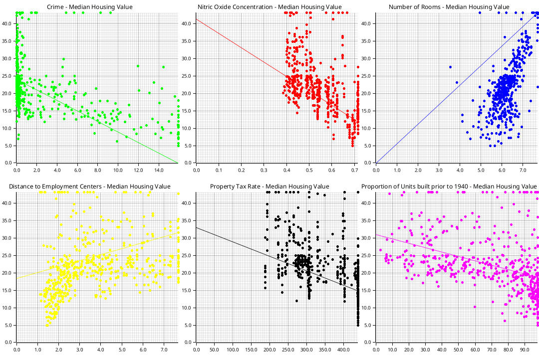
I’ll use the Boston housing dataset as an example for linear regression. The goal is to predict housing prices based on 13 parameters. The data was preprocessed by removing all samples not in the \([0.05, 0.95]\) range and by normalizing all features to the range \([0,1]\) so large features don’t overwhelm smaller ones. A few features with their optimal regression lines look like this:
Implementing the aforementioned algorithms yields the following curves for batch gradient descent and stochastic gradient descent respectively:
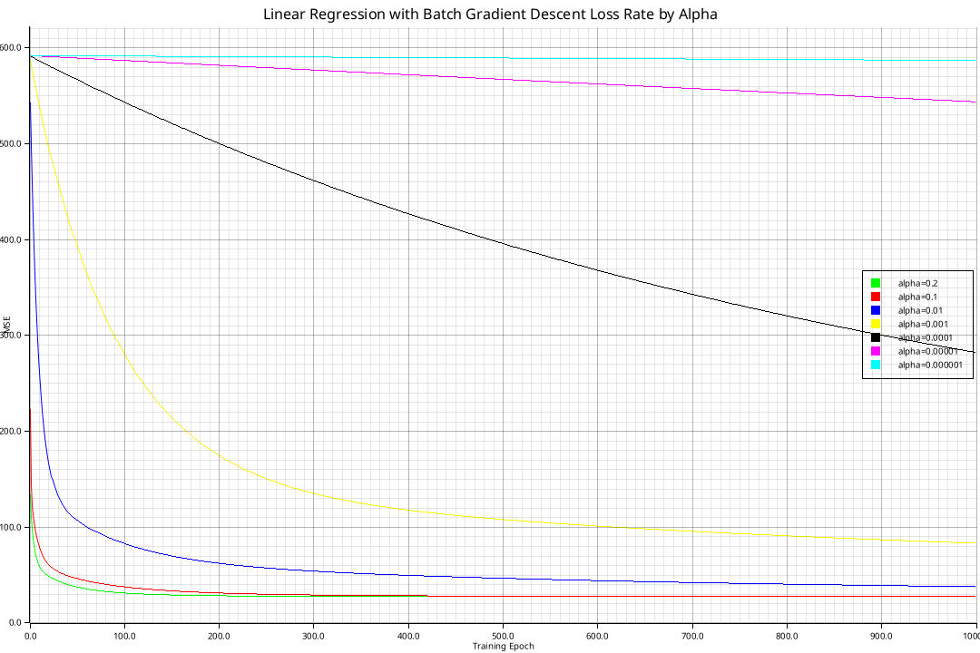
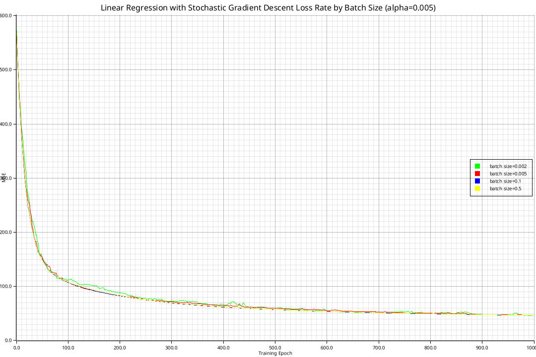
All curves converge to the minimal loss of \(21.8948\) as given by the normal equation, but some do so more quickly. Using higher learning rates than \(1\) results in divergence.
Our goal in the previous example was to predict a continuous value from a feature vector. We now turn to the problem of classification, i.e. assigning distinct classes to features. Logistic regression allows us to do binary classification in a way not too dissimilar to linear regression.
Linear regression itself is ill-suited for classification since it produces unbounded continuous values while bounded values \(h_\theta\in[0,1]\) are more desirable for obvious reasons. It also tends to deal poorly with new data and outliers. We can solve both of these problems by taking the output of the linear regression model and putting it through the logistic function \(g:\mathbb{R}\rightarrow[0,1],z\mapsto\frac{1}{1+e^{-z}}\):
\[\begin{gather} h_\theta(x)=g(\theta^T x)=\frac{1}{1+e^{-\theta^T x}} \end{gather}\]
We pursue the same strategy as before and find a maximum likelihood estimate \(\theta\). Let \(y=0\) and \(y=1\) indicate membership of \(y\) to the first resp. the second class. Assume \(h_\theta(x)\) outputs values s.t.
\[\begin{align} \Pr[y=1\vert x;\theta]&=h_\theta(x) \\ \Pr[y=0\vert x;\theta]&=1-h_\theta(x) \\ p(y\vert x;\theta)&=h_\theta(x)^y(1-h_\theta)^{(1-y)} \end{align}\]
Since \(y^{(i)}\) are assumed to be iid, the probability of observing all given outcomes \(\vec y\) given \(\vec x\) under \(\theta\) is precisely equal to the product of observing each outcome separately:
\[\begin{gather} \mathcal{L}(\theta)=p(\vec y\vert\vec x;\theta)=\prod_{i=1}^m p(y^{(i)}\vert x^{(i)};\theta)=\prod_{i=1}^m h_\theta(x^{(i)})^{y^{(i)}}(1-h_\theta(x^{(i)}))^{1-y^{(i)}} \end{gather}\]
Unfortunately, no normal equation exists for logistic regression so we resort to an iterative approach. Since we want to maximize \(\mathcal{L}(\theta)\), we can do gradient ascent which is pretty much the same as gradient descent but with a flipped sign. We will once again utilize the log likelihood \(l(\theta)=\ln\mathcal{L}(\theta)\) instead for simpler algebra:
\[\begin{gather} \theta^{t+1}\leftarrow\theta^t+\nabla_\theta\mathcal{l}(\theta^t) \end{gather}\]
Deriving the gradient:
\[\begin{align} \nabla_\theta l(\theta)&=\nabla_\theta\ln\prod_{i=1}^m h_\theta(x^{(i)})^{y^{(i)}}(1-h_\theta(x^{(i)}))^{1-y^{(i)}} \\ &=\nabla_\theta\sum_{i=1}^m \ln(h_\theta(x^{(i)})^{y^{(i)}})+\ln((1-h_\theta(x^{(i)}))^{1-y^{(i)}}) \\ &=\nabla_\theta\sum_{i=1}^m y^{(i)}\ln(h_\theta(x^{(i)}))+(1-y^{(i)})\ln(1-h_\theta(x^{(i)})) \\ &=\sum_{i=1}^m y^{(i)}\nabla_\theta\ln\left(\frac{1}{1+e^{-\theta^Tx^{(i)}}}\right)+(1-y^{(i)})\nabla_\theta\ln\left(1-\frac{1}{1+e^{-\theta^Tx^{(i)}}}\right) \\ &=\sum_{i=1}^m -y^{(i)}\nabla_\theta\ln\left(1+e^{-\theta^Tx^{(i)}}\right)+(1-y^{(i)})\nabla_\theta\ln\left(\frac{e^{-\theta^Tx^{(i)}}}{1+e^{-\theta^Tx^{(i)}}}\right) \\ &=\sum_{i=1}^m -y^{(i)}\frac{1}{1+e^{-\theta^Tx^{(i)}}}\nabla_\theta(1+e^{-\theta^Tx^{(i)}})+(1-y^{(i)})\nabla_\theta(\ln(e^{-\theta^Tx^{(i)}})-\ln(1+e^{-\theta^Tx^{(i)}})) \\ &=\sum_{i=1}^m \frac{y^{(i)}e^{-\theta^Tx^{(i)}}}{1+e^{-\theta^Tx^{(i)}}}x^{(i)}+(1-y^{(i)})(\nabla_\theta(-\theta^Tx^{(i)})-\nabla_\theta\ln(1+e^{-\theta^Tx^{(i)}}))) \\ &=\sum_{i=1}^m \frac{y^{(i)}}{1+e^{\theta^Tx^{(i)}}}x^{(i)}+(1-y^{(i)})(-x^{(i)}+\frac{1}{1+e^{\theta^Tx^{(i)}}}x^{(i)}) \\ &=\sum_{i=1}^m x^{(i)}\left(y-\frac{1}{1+e^{-\theta^Tx^{(i)}}}\right) \\ &=\sum_{i=1}^m x^{(i)}(y-g(\theta^Tx^{(i)})) \end{align}\]
This yields the following final equation (notice the similarity to linear regression):
\[\begin{gather} \theta^{t+1}\leftarrow\theta^t+\nabla_\theta\mathcal{l}(\theta^t)=\theta^t+\sum_{i=1}^m x^{(i)}(y-h_{\theta^{t}}(x^{(i)})) \end{gather}\]
Newton’s method is another iterative method which is faster in many situations. While gradient descent works by taking a small step towards the minimum or maximum, Newton’s method can be used for finding roots. Since the derivative at a minimum/maximum is equal to zero, using gradient descent on \(f:\mathbb{R}^n\rightarrow\mathbb{R}\) is equivalent to finding the root of \(f'\).
Consider the polynomial \(f(x)=x^3+0.5x^2-4x-1\). We start with some initial \(x^0\), let’s say \(x^0=0.7\). This is then updated iteratively as follows:
\[\begin{gather} x^{t+1}\leftarrow x^t-\frac{f(x^t)}{f'(x^t)} \end{gather}\]
We find the point \((x,y=f(x))\) on the graph and calculate where the tangent line cuts across the x axis. This intersection point then becomes the basis for the next iteration. The first three iterations look like this:
Seven iterations are already enough for my Python implementation to show an error value of 0.0. This methods converges quadratically, meaning after every step, the number of correct digits roughly doubles. A disadvantage compared to gradient descent is that a second order derivative is required since we want to find \(x\) s.t. \(f'(x)=0\). If we work with feature vectors \(\theta\in\mathbb{R}^n\), the mathematics stays the same, although we now need some vector calculus instead of simple derivatives: scalars are replaced by vectors and we’ll use the inverse Jacobian instead of \(f'(x)^{-1}\). More concretely, finding a root \(\theta\in\mathbb{R}^n\) for a function \(f:\mathbb{R}^n\rightarrow\mathbb{R}\) can be done as follows:
\[\begin{gather} \theta^{t+1}\leftarrow\theta^t-J_{f}(\theta^t)^{-1}f(\theta^t) \end{gather}\]
If \(f(\theta)=\mathcal{L}(\theta)\) for a loss function \(\mathcal{L}:\mathbb{R}^n\rightarrow\mathbb{R}\) whose minimum is to be found, we need to find the root of its derivative (i.e. the gradient) instead. We’ll then use the Hessian \(H\), \(H_{ij}=\frac{\partial^2\mathcal{L}}{\partial\theta_i\partial\theta_j}\) instead of the Jacobian which is the matrix of all second-order partial derivatives:
\[\begin{gather} \theta^{t+1}\leftarrow\theta^t-H_{\mathcal{L}}(\theta^t)^{-1}\nabla_\theta\mathcal{L}(\theta^t) \end{gather}\]
A somewhat simpler model is that of the Perceptron: it uses the Heaviside step function instead of a logistic curve, yielding a binary 0/1 output without any probability information:
\[\begin{align} H(z)&=\left\{\begin{array}{lr}0&z<0\\1&z\geq 0\end{array}\right. \\ h_\theta(x)=H(\theta^Tx)&=\left\{\begin{array}{lr}0&\theta^Tx<0\\1&\theta^Tx\geq 0\end{array}\right. \end{align}\]
Iterative training for a data point \((x^{(i)}, y^{(i)})\) with learning rate \(\alpha\) is done as follows:
\[\begin{gather} \theta^{t+1}\leftarrow\theta^t+\alpha(y^{(i)}-h_\theta(x^{(i)}))x^{(i)}=\left\{\begin{array}{lr}\theta^t+\alpha x^{(i)}&y^{(i)}\neq H(\theta^Tx)\\0&y^{(i)}=H(\theta^Tx)\end{array}\right. \end{gather}\]
We only update parameters when the prediction is wrong. An intuitive visual explanation can be found by looking at how an update step moves the decision boundary: consider model parameters \(\theta\in\mathbb{R}^3\) for classifying feature vectors \(x^{(i)}\in\mathbb{R}^2\) (remember we set \(x_0^{(i)}=1\) to include a bias term). The decision boundary is the set of all points \(x=(x_0, x_1)\) for which \(\theta^Tx=0\). If we plot \(x_1^{(i)}\) on the x-axis and \(x_2^{(i)}\) on the y-axis, we can get a feel for how varying \(\theta\) affect this boundary:
Solving \(\theta^Tx=0\) for \(x_2\) is simple and yields the following which might clarify the linear nature of the boundary:
\[\begin{gather} x_2=-\frac{\theta_0+\theta_1x_1}{\theta_2}=-\frac{\theta_0}{\theta_2}-\frac{\theta_1}{\theta_2}x_1 \end{gather}\]
Let’s look at a classification example and see how the boundary gets
shifted after every step to more clearly separate the two distinct
groups. We will use the HarvestTime and Weight
attributes of a Banana Quality
dataset. Green markers represent good and red markers bad quality.
We will use 500 samples in total:
Notice how the Perceptron struggles to find a boundary since the data is clearly non-separable in 2D space. We’ll later learn how this problem can be fixed. For now, let’s look at another simpler example for which such a boundary exists:
You have probably noticed how linear regression and logistic regression work in a similar fashion: they linearly combine features and then apply a function to them. They both belong to a larger class of models generalizing this notion called generalized linear models.
Before we can dive deeper and take a look at GLMs, we need to introduce something else first. If a probability distribution \(p\) can be written in the form of \(p(y;\eta)=b(y)\exp(\eta^TT(y)-a(\eta))\), it is a member of the exponential family and has some nice properties. The different terms in this case mean the following:
Let’s look at a few examples and identify the parts:
A Bernoulli experiment E has a single binary outcome of 0 or 1. If we let \(\phi=\Pr[E=1]\), it is easy to see that \(p(y;\phi)=\phi^y(1-\phi)^{1-y}\): if we let \(\phi=0\), then \(p(y;\phi)=1-y\) and if \(\phi=1\) then \(p(y;\phi)=y\). Now let’s rewrite \(p(y;\phi)\) in such a way its exponential nature becomes clear:
\[\begin{gather} p(y;\phi)=\phi^y(1-\phi)^{1-y}=\exp(\ln(\phi^y(1-\phi)^{1-y}))=\exp(\ln(\frac{\phi}{1-\phi})+\ln(1-\phi)) \end{gather}\]
It is a member of the exponential family with
A Gaussian or normal distribution is perhaps the most important distribution due to the central limit theorem: the sum of independently sampled values from any distribution approaches a normal distribution. Lots of real-world properties assume a normal distribution: age, height, IQ etc. The Gaussian is defined in terms of its mean \(\mu\) and standard deviation \(\sigma\):
\[\begin{gather} p(y;\eta=(\mu,\sigma))=\frac{1}{\sigma \sqrt{2\pi}}\exp(-\frac{1}{2}(\frac{x-\mu}{\sigma})^2)=\frac{1}{\sqrt{2\pi}}\exp(-\frac{y^2}{2})\exp(y\mu-\frac{\mu^2}{2}) \end{gather}\]
We assume a fixed variance of \(\sigma=1\) so only the mean is left as a parameter:
The Poisson distribution can be used to express the probability of a certain number of events occuring over a certain time if events occur independently and with a constant rate. If \(\lambda\) is the expected value of events observed over a certain period, then the probability observing \(n\) events is defined as follows:
\[\begin{gather} p(n;\lambda)=\frac{\lambda^n e^{-\lambda}}{n!} \end{gather}\]
For instance, if we expect to receive exactly one e-mail per hour, the probability of receiving none is equal to \(p(0;1)=\frac{1^0e^{-1}}{0!}=\frac{1}{e}\approx 0.37\). If we expect to receive exactly three e-mails per hour, the same probability decreases to \(p(0;3)=\frac{3^0e^{-3}}{0!}=\frac{1}{e^3}\approx 0.05\).
Expressing the Poisson distribution as a member of the exponential family:
\[\begin{gather} p(k;\lambda)=\frac{\lambda^ne^{-\lambda}}{n!}=\frac{1}{n!}e^{n\ln\lambda}e^{-\lambda}=\frac{1}{n!}\exp(n\ln\lambda-\lambda) \end{gather}\]
Exponential families have three particularly useful properties allowing us to estimate \(\eta\) using MLE since it is concave as well as to easily calculate the expected value and variance:
Linear regression works well if the target value has a linear relationship with the features: assuming the price of a house is roughly proportional to its size is a well-fitting assumption. This breaks down if the target doesn’t linearly respond to the features: we’ve already seen that using a linear regression model to predict probabilities doesn’t work well since the range of target values can take on many values outside \([0,1]\). GLMs on the other hand make use of a link function and appropriate distribution to relate the linear model to the target value.
Let \((x^{(i)}, y^{(i)})\) be pairs of feature-target values and assume \(p(y^{(i)}|x^{(i)};\eta)\) to be distributed according to some exponential family distribution, i.e. \(p(y^{(i)}|x^{(i)};\eta)=b(y)\exp(\eta^TT(y)-a(\eta))\). Define the output of the linear model as \(\eta=\theta^Tx\). We now relate this linear prediction to the mean of the distribution through the link function \(g\) that expresses \(\eta\) in terms of the mean \(\mu\), i.e. \(g(\mu)=\eta=\theta^Tx\). For a Gaussian, we have seen that \(\eta=\mu\) so the link function simply is \(g(\mu)=\mu\). In the case of a Bernoulli distribution, the link function is given by \(g(\phi)=\ln(\frac{\phi}{1-\phi})=\eta\). For a Poisson, we have \(g(\lambda)=\ln\lambda=\eta\).
Conceptually, the output of the model \(h_\theta(x)\) is the expected value of the distribution parameterized by the canonical parameters given by applying the inverse link function to the linear model \(\eta=\theta^T x\). Since \(g^{-1}(\eta)=\mu\) and \(\mathbb{E}[y;\eta]=\frac{\partial}{\partial\eta}a(\eta)\), this simply becomes:
\[\begin{gather} h_\theta(x)=\mathbb{E}[y;\eta=\theta^Tx]=g^{-1}(\eta)=\frac{\partial}{\partial\eta}a(\eta) \end{gather}\]

Let’s take another look at linear and logistic regression as generalized linear models:
We have already seen how errors for linear regression are assumed to be normally distributed with fixed variance. This means we have
Plotting this for the one-dimensional case: